Variational Autoencoder

In this example we will be implementing a variational autoencoder using distreqx.

Reference

bibtex @inproceedings{kingma2014auto, title={Auto-encoding variational {B}ayes}, author={Kingma, Diederik P and Welling, Max}, booktitle={International Conference on Learning Representations}, year={2014}, }

```python import equinox as eqx import jax import jax.numpy as jnp import matplotlib.pyplot as plt import optax import tensorflow_datasets as tfds from tqdm.notebook import tqdm

from distreqx import distributions ```

First, we need to create a standard small encoder and decoder module. The shapes are hard coded for the MNIST dataset we will be using.

```python class Encoder(eqx.Module): encoder: eqx.nn.Linear mean: eqx.nn.Linear std: eqx.nn.Linear

def __init__(self, key, input_size=784, hidden_size=512, latent_size=10):
    keys = jax.random.split(key, 3)
    self.encoder = eqx.nn.Linear(input_size, hidden_size, key=keys[0])
    self.mean = eqx.nn.Linear(hidden_size, latent_size, key=keys[1])
    self.std = eqx.nn.Linear(hidden_size, latent_size, key=keys[2])

def __call__(self, x):
    x = x.flatten()
    x = self.encoder(x)
    x = jax.nn.relu(x)
    mean = self.mean(x)
    log_stddev = self.std(x)
    stddev = jnp.exp(log_stddev)
    return mean, stddev

class Decoder(eqx.Module): ln1: eqx.nn.Linear ln2: eqx.nn.Linear

def __init__(self, key, input_size, hidden_size, output_shape=784):
    keys = jax.random.split(key, 2)
    self.ln1 = eqx.nn.Linear(input_size, hidden_size, key=keys[0])
    self.ln2 = eqx.nn.Linear(hidden_size, output_shape, key=keys[1])

def __call__(self, z):
    z = self.ln1(z)
    z = jax.nn.relu(z)
    logits = self.ln2(z)
    logits = jnp.reshape(logits, (28, 28, 1))
    return logits

```

Next we can construct the VAE object. It consists of an encoder and decoder, the encoder provides the mean and variance of the multivariate Gaussian prior. The output of the decoder represents the logits of a bernoulli distribution over the pixel space. Note that the Independent here is a bit of a legacy artifact. In general, distreqx encourages vmap based approaches to distributions and offloads any batching to the user. However, it is often possible to implicitly batch computations for certain disributions (sometimes even correctly). Independent is merely a helper that sums over dimensions, so even though we don't vmap over the bernoulli (like we often should), we can still sum over batch dimensions (since the event shape of a bernoulli is ()).

```python class VAEOutput(eqx.Module): variational_distrib: distributions.AbstractDistribution likelihood_distrib: distributions.AbstractDistribution image: jnp.ndarray

class VAE(eqx.Module): encoder: Encoder decoder: Decoder

def __init__(
    self,
    key,
    input_size=784,
    latent_size=10,
    hidden_size=512,
):
    keys = jax.random.split(key)
    self.encoder = Encoder(keys[0], input_size, hidden_size, latent_size)
    self.decoder = Decoder(keys[1], latent_size, hidden_size, input_size)

def __call__(self, x, key):
    keys = jax.random.split(key)
    x = x.astype(jnp.float32)

    # q(z|x) = N(mean(x), covariance(x))
    mean, stddev = self.encoder(x)
    variational_distrib = distributions.MultivariateNormalDiag(
        loc=mean, scale_diag=stddev
    )
    z = variational_distrib.sample(keys[0])

    # p(x|z) = \Prod Bernoulli(logits(z))
    logits = self.decoder(z)

    likelihood_distrib = distributions.Independent(
        distributions.Bernoulli(logits=logits)
    )

    # Generate images from the likelihood
    image = likelihood_distrib.sample(keys[1])

    return VAEOutput(variational_distrib, likelihood_distrib, image)

```

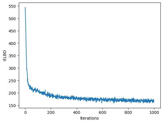
Now we can train our model with the standard ELBO. Keep in mind, here we require some vmaping over the distribution, since we now have an additional batch dimension (that we do not want to have Independent sum over).

```python def load_dataset(split, batch_size): ds = tfds.load("binarized_mnist", split=split, shuffle_files=True) ds = ds.shuffle(buffer_size=10 * batch_size) ds = ds.batch(batch_size) ds = ds.prefetch(buffer_size=5) ds = ds.repeat() return iter(tfds.as_numpy(ds))

@eqx.filter_jit def loss_fn(model, key, batch): """Loss = -ELBO, where ELBO = E_q[log p(x|z)] - KL(q(z|x) || p(z))."""

outputs = eqx.filter_vmap(model)(batch, key)

# p(z) = N(0, I)
prior_z = distributions.MultivariateNormalDiag(
    loc=jnp.zeros(latent_size), scale_diag=jnp.ones(latent_size)
)
# we need to make surve to vmap over the distribution itself!
# see also: https://docs.kidger.site/equinox/tricks/#ensembling
log_likelihood = eqx.filter_vmap(lambda x, y: x.log_prob(y))(
    outputs.likelihood_distrib, batch
)

kl = outputs.variational_distrib.kl_divergence(prior_z)
elbo = log_likelihood - kl
return -jnp.mean(elbo), (log_likelihood, kl)

@eqx.filter_jit def update( model, rng_key, opt_state, batch, ): (val, (ll, kl)), grads = eqx.filter_value_and_grad(loss_fn, has_aux=True)( model, rng_key, batch ) updates, new_opt_state = optimizer.update(grads, opt_state) model = eqx.apply_updates(model, updates) return model, new_opt_state, val

batch_size = 128 learning_rate = 0.0005 training_steps = 1000 eval_frequency = 100 latent_size = 2

MNIST_IMAGE_SHAPE = (28, 28, 1) optimizer = optax.adam(learning_rate) key = jax.random.key(0) key, subkey = jax.random.split(key) model = VAE(subkey, input_size=784, latent_size=latent_size, hidden_size=512)

opt_state = optimizer.init(eqx.filter(model, eqx.is_array))

train_ds = load_dataset(tfds.Split.TRAIN, batch_size) valid_ds = load_dataset(tfds.Split.TEST, batch_size)

losses = []

for step in tqdm(range(training_steps)): key, subkey = jax.random.split(key) batch = jnp.array(next(valid_ds)["image"]) subkey = jax.random.split(subkey, len(batch)) # val_loss, (ll, kl) = loss_fn(model, subkey, batch) # break model, opt_state, loss = update(model, subkey, opt_state, batch) losses.append(loss)

if step % eval_frequency == 0:
    key, subkey = jax.random.split(key)
    batch = jnp.array(next(valid_ds)["image"])
    subkey = jax.random.split(subkey, len(batch))
    val_loss, (ll, kl) = loss_fn(model, subkey, batch)
    # results = eqx.filter_jit(eqx.filter_vmap(model))(batch["image"], subkey)
    # plt.imshow(results.image[0])
    # plt.show()
    print(f"STEP: {step}; Validation -ELBO: {val_loss}, LL {ll.mean()}, KL \
            {kl.mean()}")

```

python plt.plot(losses) plt.xlabel("Iterations") plt.ylabel("-ELBO") plt.show()

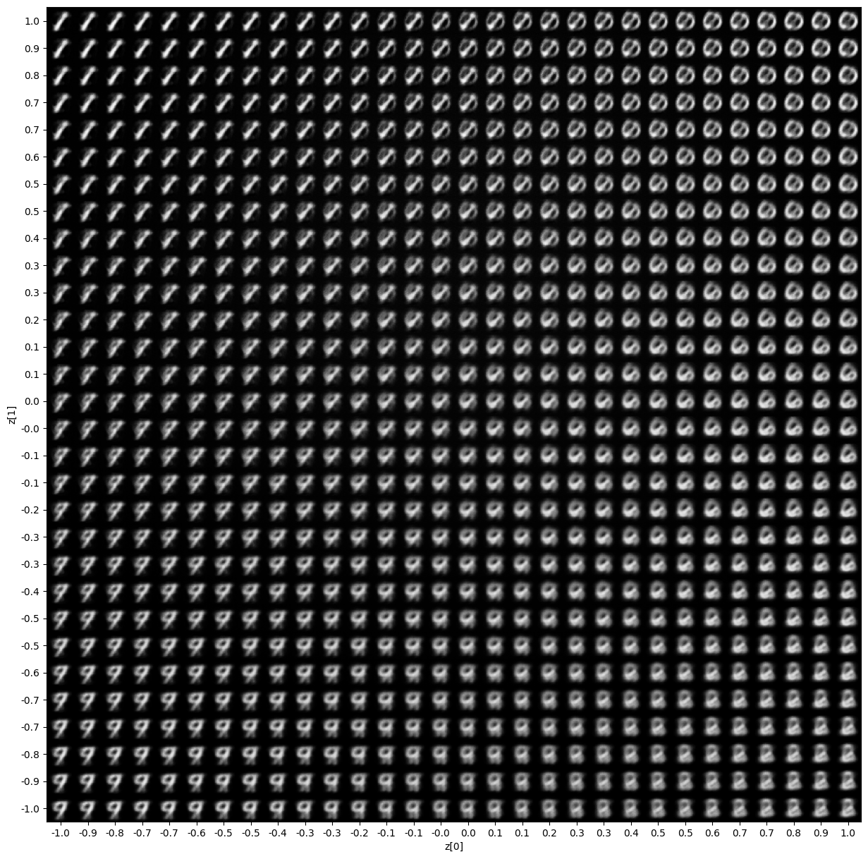
For such a small latent space, we can visualize a nice representation of the output.

```python

from: https://keras.io/examples/generative/vae/#display-a-grid-of-sampled-digits

import numpy as np

def plot_latent_space(vae, n=30, figsize=15): # display a n*n 2D manifold of digits digit_size = 28 scale = 1.0 figure = np.zeros((digit_size * n, digit_size * n)) # linearly spaced coordinates corresponding to the 2D plot # of digit classes in the latent space grid_x = jnp.linspace(-scale, scale, n) grid_y = jnp.linspace(-scale, scale, n)[::-1]

for i, yi in enumerate(grid_y):
    for j, xi in enumerate(grid_x):
        z_sample = jnp.array([xi, yi])
        # convert logits to probs
        digit = jax.nn.sigmoid(eqx.filter_jit(vae.decoder)(z_sample).squeeze())
        figure[
            i * digit_size : (i + 1) * digit_size,
            j * digit_size : (j + 1) * digit_size,
        ] = digit

plt.figure(figsize=(figsize, figsize))
start_range = digit_size // 2
end_range = n * digit_size + start_range
pixel_range = jnp.arange(start_range, end_range, digit_size)
sample_range_x = jnp.trunc(10 * grid_x) / 10
sample_range_y = jnp.trunc(10 * grid_y) / 10
plt.xticks(pixel_range, sample_range_x)
plt.yticks(pixel_range, sample_range_y)
plt.xlabel("z[0]")
plt.ylabel("z[1]")
plt.imshow(figure, cmap="Greys_r")
plt.show()

plot_latent_space(model) ```

```python

```